In 2021 I put out a working paper with my simple mathematical model that illustrated MMT’s theory of the determination of the price level. You can read the paper here, or an earlier version of the model in a blog post here. Then at the 2nd MMT Summer School in Poznań, none other than Steve Keen did a demo of his Minsky modeling software, and it occurred to me that it would be fairly easy to set up my model in Minsky. So I did it, and I’m going to show you the results in this post.
A word of warning: this is not going to be an introduction either to the model, or to the Minsky software. So, my apologies, but this post is for a bit of a niche audience! If you want to get all the details here, then I’d encourage you to read about the model first, and maybe watch a few minutes of one of Steve’s video demos of Minsky. My primary purpose I’d say is to review my experience with using Minsky, and also to note a few changes I made to the model since its last edition.
It did turn out to be quite easy, and the whole process took maybe 2.5 hours. For the first half of this post I am going to discuss in detail the changes I had to and chose to make to the model. If you’re not interested in the technical details there, feel free to skip to the second half where I’ll show the final outcome of the model in Minsky!
The Changes
Discrete to Continuous Time
The first change was required by the software, and it was changing the model from discrete time to continuous time. That is, originally, the model had time coming in discrete chunks, starting in period 1, then moving to period 2, then 3, and so on, where maybe we suppose that each of these corresponds to, say, one month or one quarter. But Professor Keen has not built an option for discrete time into Minsky. (I asked him about this, and he said that he believes that continuous time models are better and that economists should switch over, so this is his way of nudging people in that direction. FWIW I don’t have strong feelings about discrete time vs. continuous time.)
For most of the equations this was pretty simple, where the “change” in a variable just becomes the “rate of change” of that variable, so from a discrete difference to a derivative. And actually, the Godley Table functionality does this for you automatically for the stock variables, like household wealth. That’s great.
The one variable where it was less trivial was for the price adjustment process.
In the discrete time version of the model, the new price level is determined by taking the previous price level and multiplying it by a number, where that number is determined by the supply/demand situation in the market. If that number is bigger than 1 then prices go up, and this corresponds to excess demand; if that number is between zero and 1, then prices go down, and this corresponds to excess supply, or prices being bargained down. I did not do this previously, but here I am referring to that number as the “pressure.” We can also throw in a constant that scales the pressure, affecting how strongly prices react to imbalances. So then the final equation is that the ratio of new price to old price is equal to the pressure times the scale constant.
In the continuous time version, “the ratio of new price to old price” becomes the continuous percent rate of change, or the derivative of the price divided by that price.
When I say this was less trivial, what I mean is a) I had to think about that for a few minutes, and b) I had to figure out how to do it in Minsky. As far as I can tell, you can’t directly set a derivative of a variable to be equal to things, and instead you have to use an integral. So, to define the price variable, I took the pressure times the scale constant, divided by price, and then integrated it. That looks like this:

Right-Siding Up!
I view my original paper as serving a number of functions. For one, it helps formalize long-time MMT insights. Another, it serves the social function of getting critics of MMT off our backs — I‘ve lost count of how many times I’ve had this interactions: somebody says to me “where’s your model?!” then I say “here’s one,” and then I never hear from them again. That’s at least been nice for demonstrating that most people demanding models never seriously intended to spend the time to read one.
Another thing it did that I found important was that it very intentionally flipped standard logic on its head in a number of ways, particularly that it didn’t bother modeling the “real” part of the economy at all, only looking at the supply and demand for net financial wealth (“money”). There’s of course nothing new about doing money supply and money demand, but centering the entire model around that is unusual — if you look at models in mainstream monetary economics textbooks, they start the way all the rest of them do, with an agent maximizing consumption, and everything in “real” terms. My model, by contrast, begins with the nominal to explain the nominal.
But, unsurprisingly, that does make it hard to keep straight. This is why the paper is filled with repetitive parentheticals along the lines of “sellers of money (buyers of goods) meet buyers of money (sellers of goods)” and the like. Confusing.
So, when I presented the model again in Poznań, I wanted to try flipping this back to the normal way-around. That means the variables in the model become the quantity of labor supplied and the quantity of labor demanded, and prices become the usual how-many-dollars-to-buy-a-good rather than how-many-goods-to-buy-a-dollar.
Quantity of labor supplied then is just constant. This is how things work in the backwards-L “Keynesian” aggregate supply curve: the economy has some amount of capacity. Quantity of labor demanded depends on private wealth, but adjusted for price (whereas in the paper, it’s the supply of money to be sold that depended on the amount of wealth in dollar terms — these are the same thing but from different angles).
Speaking of private wealth,
Godley Tables
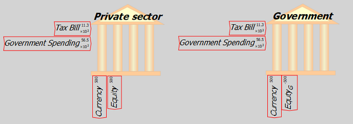
One feature of Minsky is its ability to keep track of accounting for you, through something called a Godley Table. In my little toy model, there’s not much accounting to lose track of, but this is handy nonetheless, as it generates equations for you automatically. The symbols look like this:

And let’s look at one of the tables opened up, say, the private sector:

This is showing you that there’s just one asset, currency, and no private liabilities. This is matched by private equity. This also shows you the two actions that can change private sector holdings of currency/equity: when the private sector pays taxes it loses currency, and when it sells labor to the government it receives currency.
Because the Godley Table forces the model to be balance sheet consistent, there’s a set of new variables that aren’t in the paper, representing the net wealth of the private and government sectors. I can see two ways to understand why they’re not in the paper. One argument could be that they are there, just in the background and they go un-modeled because they don’t affect the rest of the modeled world. The other argument would be that there is nothing else in the background in the model, and so net wealth just equals the stock of currency, since (for the private sector) that’s the only asset and there are no liabilities. I like the first explanation better, but the second one probably makes more sense. Either way, it’s just philosophical.
Scaling imbalance terms
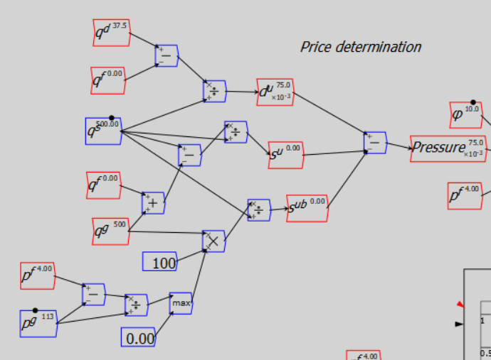
Finally, another technical change from the paper is that I decided to scale the market-imbalance terms that make up the “pressure” indicator. I do this by dividing them through by quantity -supplied. This makes each term a measure of the imbalance as a percent of the market. This is a subtle change, but makes the model more sensibly scale-invariant: eg. if the market is in shortage by 2 units, it seems like prices should go up faster if the total size of the market is 10 units rather than 10,000 units.
The Model
Ok, technical details aside, let’s at last get to the results. Here’s a zoomed out shot of the whole thing:

The primary segments are 1) where the transaction outcomes are determined:

2) Where tax revenue is determined, which requires determining total spending by sector:

And 3) where the price mechanism happens. I showed the bit with Pressure above, so here’s where the imbalances that make it up happen:

The last bit is the graphs, for actually watching the simulations. Here’s the results of a trial run:

The message of the model is in the top left graph, where the red line is the private price level while the green line is the price the government offers to pay when it spends. As shown, if the red line starts away from the green line, it will head over time back to the green line, meaning in the steady-state, market prices come to equal the government’s exogenous price level. In the chart, once this happens, I then ‘shock’ the model by reducing the government’s price, so that the green line jumps down, and we see that the red line starts heading down to meet it. Once this happens, I think shock the model again by increasing government prices, so that the green line jumps up, and we can see that the red line again converges toward it.
If you like, you can figure out why this happens by observing causal mechanisms which are shown in the other three graphs. One element that’s critical is that if the government is paying below-market prices, then nobody will sell to the government so government spending drops to zero. But with taxes still non-zero, this drains private financial wealth, eventually reducing private demand and prices, until they come back into line with the government’s price level. On the other hand, when the government is paying above-market prices, then everybody wants to sell to the government, driving shortages in private markets while causing government spending to soar, which further adds to private financial wealth, demand, and private prices.
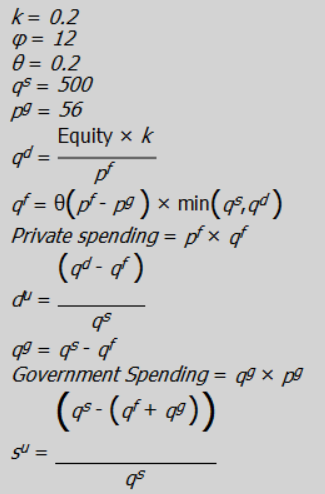
Finally, for people into equations, here are the equations for the model, that are generated by the software based on how the blocks are wired up:


The parameter values are more or less arbitrary, with a few exceptions. First, the private and government prices only converge if the tax rate is positive. If you set the tax rate to zero, then these markets become completely disconnected. That’s an essential lesson of the model: the government’s pricing power over its currency is predicated on its ability to enforce taxes, which drain the currency from circulation and so force people to sell goods to the government at government prices. I discuss this in detail in the paper. The other constant that really matters is the pressure constant: if it’s too large, prices become too reactive to tiny disturbances, and the model starts acting very strangely — you can get bizarre stuff like oscillation or negative prices. This is typical for models like this.
Conclusion and Review
All in all, I found the software to be quite easy to use, although it’s a bit rough around the edges. The wiring interface makes it really easy to start building models very quickly, and Steve’s presentation videos where he basically improvises entire models on-the-fly are a testament to this.
My main complaint would be that the documentation needs work. Also I don’t share the opposition to discrete time, so I wouldn’t mind a discrete time option.
Another issue is that the sliders to adjust the parameters manually are really small, which makes them hard to control. It would be great if there was a way to get a bigger slider, detached from the block of the parameter it’s controlling. Also, the display for numbers doesn’t always make much sense. For example, the tax rate here is allowed to vary from zero to one in increments of 0.05, but Minsky insists on showing me the number in scientific notation, which is a little annoying.

I will definitely praise Minsky for improving on its stability — I first tried to use Minsky maybe 5 years ago, but didn’t get very far because it kept crashing! This seems to have been solved now.
Building the model this way actually did teach me a few things about how it worked, so that’s cool. I think that simulating a model is an extremely useful tool for understanding its dynamics, even a simple model like this one here, and Minsky is a nice tool for doing this. I definitely recommend giving Minsky a try if you’re playing around with a model that it’s amenable to.
Finally, if you’re interested in playing around with my model in Minsky, let me know and I can send you the file. Cheers!